How to index the cognitive difficulty of exercises with the using-explaining taxonomy

Version 2.0

1 - What is this document, in brief

This taxonomy is designed to index the cognitive difficulty of exercises and questions in engineering courses along two independent dimensions:

the “using” dimension, to index the cognitive difficulty of solving a problem using specific tools, e.g., formulas, algorithms, and design procedures; and
the “explaining” dimension, to index the cognitive difficulty of explaining concepts or claims via reasoning, connecting, illustrating or proving something.

This document illustrates the taxonomy itself, plus how to find which taxonomy level an exercise has, assuming that the person doing this labelling has one or more alternative correct solutions to the exercise being labelled.

2 - Some nomenclature

This manual gives to the following words the following meanings

content unit: an atomic unit of knowledge, e.g., “electric potential”, “Rouché - Capelli theorem”, “matrix - vectors multiplications”, etc. For a more verbose explanation of this concept, and for instructions on how to define the list of content units that are taught in a subject, please refer to the associated manual.
skill: the ability to apply knowledge and use know-how to complete tasks and solve problems. The here proposed using-explaining taxonomy assesses the mastering levels of some skills in this sense: “a person masters the skills <list of content units> at a using-explaining level <list of levels>” means that that person can correctly answer questions related to that content units through solutions that have been labelled as being at that using-explaining taxonomy levels or easier. As a shorthand, we also say that in this case “the student masters that content units at that taxonomy level”.
competence: the ability to use knowledge, skills and personal, social and / or methodological abilities in a responsible and autonomous way, in work or study situations and in professional and personal development. For now the using-explaining taxonomy does not assess the mastering levels of competences. In a sense, this taxonomy for now refers only to contents.

3 - An overview of how to label an exercise in terms of using-explaining taxonomy levels

Looking at the process of labelling an exercise with a bird-eye view, the strategy:

Assumes that, together with the exercise, the person doing this labelling is given one or more alternative solutions to the exercise;
Requires that for each of these solutions the labeller:
a) first indexes each solution in terms of its “using” taxonomy level (more information in section 4)

b) then indexes it in terms of its “explaining” taxonomy level (more information in section 5)

c) finally indexes it, if desired, in terms of its expected time requirements (more information in section 6)

Note thus that the indexing of the exercise is actually the indexing of its known solutions! Note also that the using and explaining dimensions are modeled as independent, thus they should be assessed independently.

Importantly, once a person has familiarized with sections 4, 5 and 6 then that person may perform the labelling process using the questionnaire / algorithm in section 7.

4 - The potential taxonomy levels of a solution along the “using” dimension

level “using 0” solutions: solutions that neither involve computing numerical results, nor require using formulas, algorithms, or design/analysis procedures. “Using 0” solutions are thus solutions that connect, illustrate or prove concepts or claims just through reasonings and that, e.g., involve no numerical computations at all.
level “using 1” solutions: solutions that solve the exercise by straightforwardly applying just a formula / algorithm / methodology that is mentioned in the formulation of the exercise, and nothing more. Typically “using 1” solutions are the most-immediate and simplest answers to exercises that ask the students something like “apply this formula or algorithm to compute this result”. “Using 1” solutions involve thus neither creativity nor using something that was not explicitly mentioned, but instead only memory recalling operations about how to use these things that are mentioned and how to perform computations, potentially without even needing to understand what one is doing. Note that actual understanding or abilities to explain the underlying reasonings are indexed through the dimension “explain”, as detailed in section 5.
level “using 2” solutions: solutions that compute the numerical results asked by the exercise by applying mechanically a series of formulas and algorithms in a reasonably standard way, i.e., without creating anything new, but where some of these ingredients are not explicitly mentioned in the formulation of the exercise. Typically “using 2” solutions are solutions that require thinking about “what” to use, because the exercise does not list all the ingredients contained in that solution or mentions more information than needed, but do not require creativity on “how” to use these ingredients because they follow typical patterns. In other words, they are solutions that put together a series of formulas and algorithms in a semi-mechanical fashion.
level “using 3” solutions: solutions that as in “using 2” require using ingredients that are not explicitly mentioned in the formulation of the exercise (and thus thinking at “what” to use), but that also require creativity in using such ingredients. Typically “using 3” solutions are solutions that require thinking simultaneously about what to use, how, and why. This means that there exist some intermediate steps of the solution that require the student to have understood the meanings & implications of what she/he is doing, otherwise that person wouldn’t understand how to proceed. Also, such questions may require the student not to fall for typical “pitfalls”.

5 - The potential taxonomy levels of a solution along to the “explaining” dimension

level “explaining 0” solutions: solutions that do not include any type of communication of contents (i.e., recognizing, connecting, illustrating or proving something in words, pictures, or similar). Typically “explaining 0” solutions are solutions that involve only algebraic manipulations, numbers, or symbols, and as such may be provided even by persons that do not understand the meaning of the operations they are executing (like, “compute the determinant of this matrix”). Note that solutions referring to exercises like “define this concept” are “explaining 1” even if they may be written just with symbols. Also solutions to multiple choice questions may be “explaining 1”, or “explaining 2” even if they do not involve verbalizing something (cf. below)
level “explaining 1” solutions: solutions that include the reproduction of basic knowledge such as recalling statements, definitions, properties, schemes, etc., about contents that are explicitly asked in the body of the exercise / question. Typically “explaining 1” solutions are merely defining or recalling something specific, or recognizing what are correct keywords / phrases which define the contents mentioned by the exercise. Thus “explaining 1” solutions do not require thinking about / understanding what is the meaning, implication or usefulness of the to-be-verbalized.
level “explaining 2” solutions: solutions that include the communication of knowledge such as contextualizations, reasonings, connections, and similar higher level cognitive operations that require not only memory recalling but also understanding. They do not require creative processes and are carried out within that content units that are explicitly mentioned or clearly hinted at in the body of the exercise. Thus “explaining 2” solutions require thinking at what is the meaning, implication or usefulness of the to-be-communicated, but somehow are “within the box”.
level “explaining 3” solutions: solutions that include communicating knowledge that requires leveraging ingredients that are not obvious from the formulation of the exercise, and that demonstrate creativity, realization, personal reflection or understanding. Thus “explaining 3” solutions do not only connect ingredients, but also find and make use of connections with concepts not mentioned or hinted by the exercise, potentially also from other fields, to realize something, reflect on something, or create something new. “explaining 3” solutions show thinking outside of the box, and are typically associated to exercises for which there is not necessarily a single correct answer and for which reasoning may include arguments about opinions.

5.1 - Clarifying the hierarchies among the taxonomy levels above

Higher taxonomic levels along one dimension implicitly include all the lower levels along the same dimension. For example, if a solution is “explaining 2” then it includes “explaining 1”, since it also directly or indirectly requires memory recalling operations even though this might not be explicitly mentioned in the solution. Note that this implicitly justifies the validity of saying “a person masters the skills <list of content units> at a using-explaining level <list of levels >”.
Moreover the two dimensions of “using” and “explaining” are intended to be independent. This means that a solution may be “using 0 and explaining 3”, others may be “using 1 and explaining 0”, even if these solutions tend to be not common. There are however certain combinations that are unlikely to occur such as “using 3 and explaining 0” as creative solutions usually involve the explanation of some theory.

6 - Adding ancillary information about a solution

If desired, users may also index how long it should take for a student mastering that subject to find and lay down that specific solution with pen and paper (if there is no clear indication that the solution should be laid down in other ways – in that case, the time it should take to do in the suggested way).
Note that this is a rather subjective indication: typically the more complex the solution (i.e., the more content units are employed, and the higher its using-explaining taxonomy levels are), the less accurate this time indication will be.
This information may enable interested users in doing advanced searches in the portal (e.g., “portal please create an exam lasting a certain amount of time, involving these content units at these taxonomy levels”).

7 - “How do I label my solutions?” A step-by-step algorithm to do the labelling

The following algorithm is a sort of dynamic questionnaire that helps users to assess the taxonomy levels of the solutions they wish to assess. The .tex sources to generate this image are in this Overleaf

QUESTIONS FOR THE “USING” PART

ANCILLARY QUESTION [QA.a] What is the minimum expected amount of minutes it should it take for a student that knows how to reproduce this solution perfectly to actually write it down with pen and paper? (Or to do it in the way the exercise asks to?) If you think you cannot give a good indication of this, skip this part. If you think you can then set t and then exit

OTHER SANITY CHECKS (these are performed automatically by the portal)

If u == 0 && e == 0: ERROR: this is impossible;

if u == 3 && e == 0 WARNING: there is a too big difference between u and e;

if u == 0 && e == 3 WARNING: there is a too big difference between u and e.

Examples of how to identify the taxonomy levels of an exercise

intuition: for multiple choice questions it would be better to create questions that have only one solution path, and do questions for which there is only one correct answer (not multiple ones)

Example 1: “using 1, explaining 0”
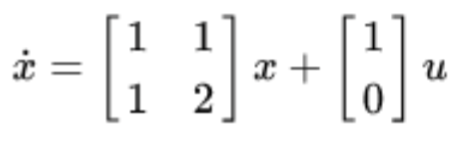
Exercise: Consider the open-loop system Use Ackermann's formula to determine a state feedback matrix that allocates the poles of the closed loop system into -5 and -6.
Solution: (and all the equations / computations associated to this)
Assessment of the solution through the questionnaire: QU.a yQU.b yQU.c nQE.a n→ u1 e0

Example 2: “using 2, explaining 1”
Exercise: let h(t) = 2 for t in [0,2), 0 otherwisebe an impulse response. Draw the forced response associated to this LTI systemand corresponding to the inputu(t) = 1 for t in [1, 2) and [2, 3), 0 otherwise.
Solution: the solution draws the impulse response, draws also the input, then draws how the convolution is at some relevant point, and then plots the corresponding forcedresponse starting from the result of the convolution at the relevant points
Assessment of the solution through the questionnaire: QU.a y QU.b n (it uses also convolution) QU.d y QU.e n QE.a y QE.b y QE.c y → u2 e1

Example 3: “using 0, explaining 3”
Exercise: determine whether the input-output impulse response of a SISO LTI system that admits more than one output-equilibrium in free evolution can be theimpulse response of a BIBO stable system or not.
Solution: if the LTI has more than one output equilibrium in free evolution it means that the IO impulse response does not decay to zero, since asymptotically it must be that y(t -> \infty) = c y_0. This means that the impulse response is not absolutely integrable, thus the system cannot be BIBO
Assessment of the solution through the questionnaire: QU.a n QE.a y QE.b n QE.d n QE.e y → u0 e3

Example 4: “using 0, explaining 1”
Exercise: What do the values of the coefficients of the impulse response of a finite impulse response filter represent?
Solution: they represent the coefficients of the moving average filter y = ‘moving average of the last N values of the input”
Assessment of the solution through the questionnaire: QU.a n QE.a y QE.b y QE.c y → u0 e1

Example 5: “using 0, explaining 2”
Exercise: Explain why the following discrete-time system y(k+1) = - y(k) + x(k)with input x and output y represents an infinite impulse response filter.
Solution: because its transfer function is so that there is a pole and then if we antitransform the transfer function we get an infinitely long impulse response
Assessment of the solution through the questionnaire: QU.a n QE.a y QE.b n QE.d y QE.e n → u0 e2

Example 6: “using 2, explaining 1”
Exercise: Three periodic time signals xi(t) and their corresponding Fourier series coefficients Dj[n] are illustrated below in a random order. Which Fourier series coefficients plot Da[n], Db[n], Dc[n] associates to which signal x1(t), x2(t), x3(t)? Motivate your choices.
Solution: do the association looking at the amplitude of frequency of each sinusoid, plus checking whether there is an offset or not (ie a DC component). Thus 2nd on the left → 3rd on the right, 1st on the left → 1st on the right
Assessment of the solution through the questionnaire: QU.a n QE.a y QE.b n QE.d y QE.e n → u0 e2

Example 7: “using 0, explaining 3”
Exercise: Find a typical example where a finite impulse response filter is used and argue why this filter type is chosen instead of an infinite impulse response filter.What would be the risk, consequence or effect of choosing an infinite impulseresponse filter in this example?
Solution: finite impulse response filters are always stable as they have no poles (or only poles in the origin of the z-plane). Hence, for filter problems where stability is of utmost importance and a sharp transitions between stop band and pass band are needed, using an infinite impulse response filter would entail the risk of having unstable poles (due to small inaccuracies in implementing the poles on a system with quantised coefficients) as the number of poles / order of the system might have to be chosen very high to achieve the desired high roll-off. Here, in order to avoid such potential instabilities, an FIR filter with sufficiently high order could and should be used.
Assessment of the solution through the questionnaire: QU.a n QE.a y QE.b n QE.d n QE.e y → u0 e3